1. The Problem

Before getting into GPU parallelization, let's start with the problem that led us there. We had an ML inference workload with a strict end-to-end time requirement. As the amount of data and number of processing steps grew, simply making the model faster wasn't enough. A substantial part of the execution time was being spent in the stages leading up to inference. When we profiled the workload, the preprocessing stage stood out as an obvious place to investigate. It was largely CPU-bound and relied heavily on Pandas and NumPy. That raised a fairly straightforward question:

If we already have a GPU available, can we use it to accelerate the preprocessing as well?

The first approach was exactly what you might expect: replace CPU-oriented operations with CUDA-enabled alternatives, moving from Pandas → cuDF and NumPy → CuPy wherever possible.

It sounds simple.
It wasn't.

The interesting part wasn't getting the code to run on the GPU. It was figuring out when moving computation to the GPU actually made the pipeline faster.

2. The Pipeline

At a high level, the pipeline looked like this:

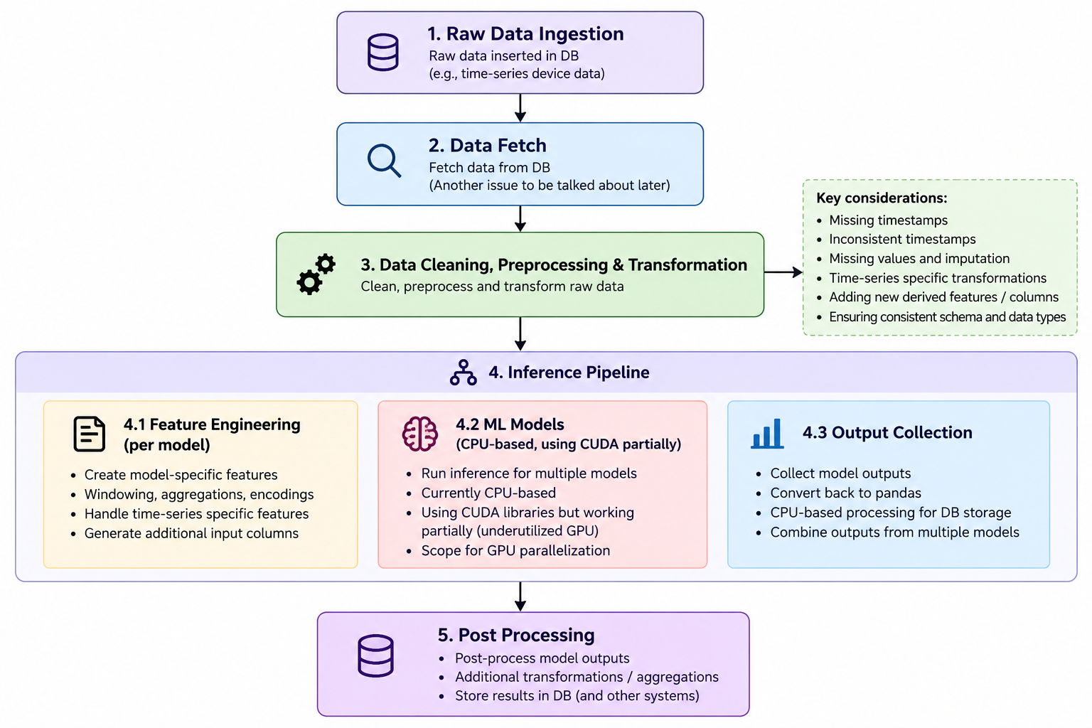
The data was time-series data associated with many unique IDs.
That made preprocessing more complicated than a simple collection of independent rows.

We had to deal with things such as

missing timestamps
irregular observations
missing values
feature transformations
model-specific preprocessing

The interesting part was figuring out which of these operations were actually good candidates for parallel execution.

3. The First Attempt: Pandas + NumPy → GPU

A lot of the existing preprocessing code was written using Pandas and NumPy.

The obvious first step was to look at CUDA-enabled alternatives.

For example, imagine we have 10 million rows:

import pandas as pd
import numpy as np

df = pd.DataFrame({
    "value": np.random.rand(10_000_000),
    "temperature": np.random.rand(10_000_000) * 100,
    "humidity": np.random.rand(10_000_000) * 100
})

# Feature engineering
df["normalized_value"] = (
    df["value"] - df["value"].mean()
) / df["value"].std()

df["heat_index"] = (
    df["temperature"] * 0.7 +
    df["humidity"] * 0.3
)

df["anomaly_score"] = np.abs(
    df["normalized_value"]
)

df["is_anomaly"] = df["anomaly_score"] > 2

Conceptually, the computation is happening on the CPU:

RAM --> NumPy / Pandas --> CPU --> Result

Now consider moving the dataframe and numerical operations to the GPU using RAPIDS cuDF and CuPy.

import cudf
import cupy as cp

df = cudf.DataFrame({
    "value": cp.random.rand(10_000_000),
    "temperature": cp.random.rand(10_000_000) * 100,
    "humidity": cp.random.rand(10_000_000) * 100
})

df["normalized_value"] = (
    df["value"] - df["value"].mean()
) / df["value"].std()

df["heat_index"] = (
    df["temperature"] * 0.7 +
    df["humidity"] * 0.3
)

df["anomaly_score"] = cp.abs(
    df["normalized_value"].values
)

df["is_anomaly"] = df["anomaly_score"] > 2

Now the data and computation can remain primarily in GPU memory:

                  GPU VRAM
              ┌───────────────┐
              │ value         │
              │ temperature   │
              │ humidity      │
              └───────┬───────┘
                      │
                      ▼
                     GPU
                      │
                      ▼
                  Results

For sufficiently large operations, this can be significantly faster.

But this is where I learned an important distinction.

4. GPU-Friendly Does Not Mean "Everything Is Faster"

For a large enough workload, operations such as element-wise arithmetic, reductions, aggregations, transformations, matrix operations can benefit substantially from GPU parallelism.

But the size and structure of the operation matter.

If an operation is tiny, the GPU may have very little useful work to do.

You might see something like:

CPU operation --> small runtime
GPU operation --> slightly smaller runtime

When measured individually, the GPU version may be faster.

But when the operation is only a tiny fraction of the complete pipeline, that difference may barely move the end-to-end runtime.

This was one of the first lessons I learned:

A faster individual operation does not automatically mean a meaningfully faster pipeline.

For our workload, the interesting gains came from finding large, repetitive computations where the GPU had enough work to justify its parallel execution model.

Moving computation to the GPU isn't the same as parallelizing it

There is another trap here.

Just because we move our data and computation to the GPU doesn't mean that the computation itself has suddenly become parallel.

Consider a simple cumulative calculation:

result = np.zeros(len(data))

for i in range(1, len(data)):
    result[i] = result[i - 1] + data[i]

The dependency looks like:

result[0] -> result[1] -> result[2] -> result[3] -> ...

We could move the data to the GPU:

data = cp.asarray(data) result = cp.zeros(len(data))
for i in range(1, len(data)):
    result[i] = result[i - 1] + data[i]

Now the data lives on the GPU, but the fundamental dependency hasn't changed.

i = 1 → calculate 
       ↓ 
i = 2 → calculate 
       ↓ 
i = 3 → calculate 
       ↓ 
...

The GPU is being used, but we haven't given it the kind of independent workload where its parallel execution model can really shine. This distinction became important for our time-series preprocessing.

5. Where the GPU Really Shines: Matrix Operations

A good way to see why GPUs are powerful is matrix multiplication.

Consider:

C = A @ B which is basically how we multiply matrices in python. Its the same as: cp.matmul(A, B)

Suppose:

A = 10,000 × 10,000
B = 10,000 × 10,000

Conceptually, every element of C is computed from a row of A and a column of B:

C[i][j] = Σ A[i][k] × B[k][j]

There are a huge number of these calculations. And importantly, many of them can be computed independently.

Conceptually:

                    Matrix C

              C[0,0] C[0,1] C[0,2] ...
                 │      │      │
                 ▼      ▼      ▼
               Work   Work   Work
                 │      │      │
                 └──────┴──────┘
                       GPU

This is exactly the kind of workload GPUs are designed to attack.

Instead of one CPU core calculating each result sequentially, the GPU can distribute enormous amounts of similar arithmetic across its execution resources.

For operations like this, the GPU is not merely doing the same work "a little faster." It is exploiting a fundamentally different execution model:

Many threads performing similar operations over large amounts of data.

That is where GPU parallelization starts becoming really powerful.

6. The Hidden Problem: Data Movement

There is another factor that has to be considered when moving CPU-based preprocessing to the GPU: data movement. If the data repeatedly moves between CPU memory and GPU memory, we can end up with:

CPU
 │
 │ transfer
 ▼
GPU
 │
 │ computation
 ▼
CPU
 │
 │ transfer
 ▼
GPU
 │
 │ computation
 ▼
CPU

That overhead is real.

However, in our workload, this was not the primary bottleneck once we started working with sufficiently large operations.

If moving a large dataset takes an additional second or two, but we save tens of seconds or minutes in the computation itself, that transfer cost is relatively small.

The important distinction is therefore not:

"Never move data between CPU and GPU."

It is:

Avoid unnecessary transfers when the computation is too small to justify them, and make the GPU work large enough that the computational savings dominate the transfer overhead.

In our case, the bigger problem was not simply that data had to move once.

The problem was repeatedly switching between CPU-oriented and GPU-oriented representations across small pieces of work.

7. The Next Question: Can We Batch More Work?

Once we understood that the GPU needs enough useful work, another question became important:

Are we giving the GPU enough data at once?

Part of the workload was being processed in chunks:

Chunk 1 → GPU
Chunk 2 → GPU
Chunk 3 → GPU
Chunk 4 → GPU
...

Instead, where the computation allowed it, we wanted to move toward:

Large batch
    │
    ▼
   GPU
    │
    ├── operation
    ├── operation
    ├── operation
    └── operation

The intuition was simple:

More independent work gives the GPU more opportunity to stay busy.

But this introduced another problem. We had workloads where a large amount of data needed to be processed at once. In trying to make these operations more suitable for the GPU, we were sometimes converting them into larger matrix-based operations. While this exposed more parallelism, it also increased the memory footprint considerably. At that point, VRAM became the bottleneck, and the GPU was spending more effort dealing with memory pressure than doing useful computation.

This became particularly relevant when multiple processes were sharing the same GPU, so it is less important for the single-instance case we're focusing on here. Still, it highlights an important consideration when moving larger workloads to the GPU: GPU memory is a finite resource.

A practical way to handle this is to understand the memory requirements of your workload, determine the amount of data the GPU can comfortably process, and introduce batching when necessary.

8. The Problem With Time-Series Dependencies

Our workload involved time-series data, and time-series operations can contain dependencies between observations.

Imagine:

A → B → C → D → E

where:

B = f(A)
C = f(B)
D = f(C)
E = f(D)

We cannot simply treat this as:

A   B   C   D   E
↓   ↓   ↓   ↓   ↓
f   f   f   f   f

because C depends on the result of B, D depends on C, and so on.

This led to an important distinction:

The amount of data is not the same thing as the amount of parallelism.

A dataset can contain millions of rows while parts of its computation remain sequential or dependent.

So instead of asking:

"Can this entire operation run on the GPU?"

we started asking:

"Which parts of this operation are actually independent?"

That was a much better question.

9. Making the Time-Series Data More Regular

One of the preprocessing steps was creating a consistent time grid for each unique ID. Suppose the original observations looked like:

10:00 → 12
10:03 → 15
10:07 →  9

We could create a complete timeline between the minimum and maximum observed timestamp:

10:00 → 12
10:01 → ?
10:02 → ?
10:03 → 15
10:04 → ?
10:05 → ?
10:06 → ?
10:07 →  9

So, it would look somewhat like this:

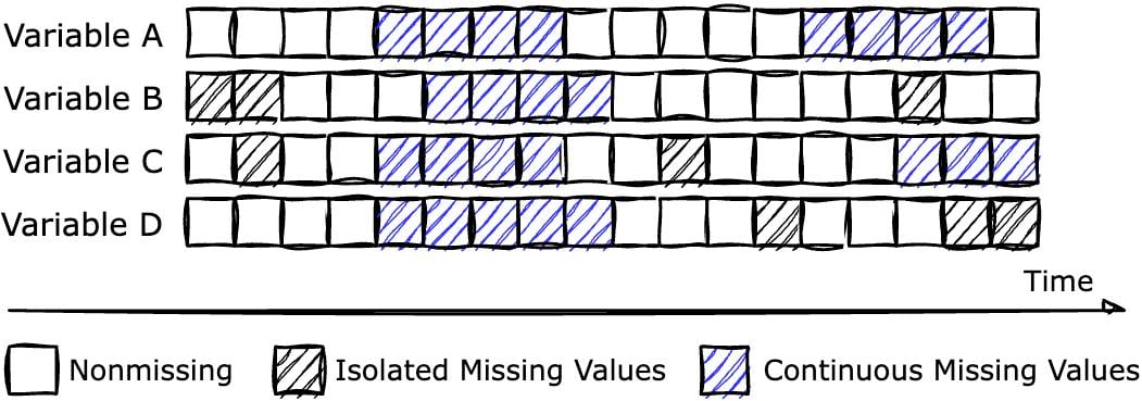
For the newly introduced or unavailable values, we can use an indicator or another column to represent that this is an imputed value, or synthetic value.

Once the time grid was regularized, the imputation logic for the newly created timestamps could be applied consistently for each unique ID.

At first glance, imputation can look like extra processing. If a value is missing, why not just leave it missing?

The problem is that missing data can change how our model interprets the underlying signal. In a time-series workload, gaps aren't just empty cells. They can change the shape, continuity, and patterns that our ML models learn from.

You can see how dramatically this can change our interpretation of the data in the chart below.

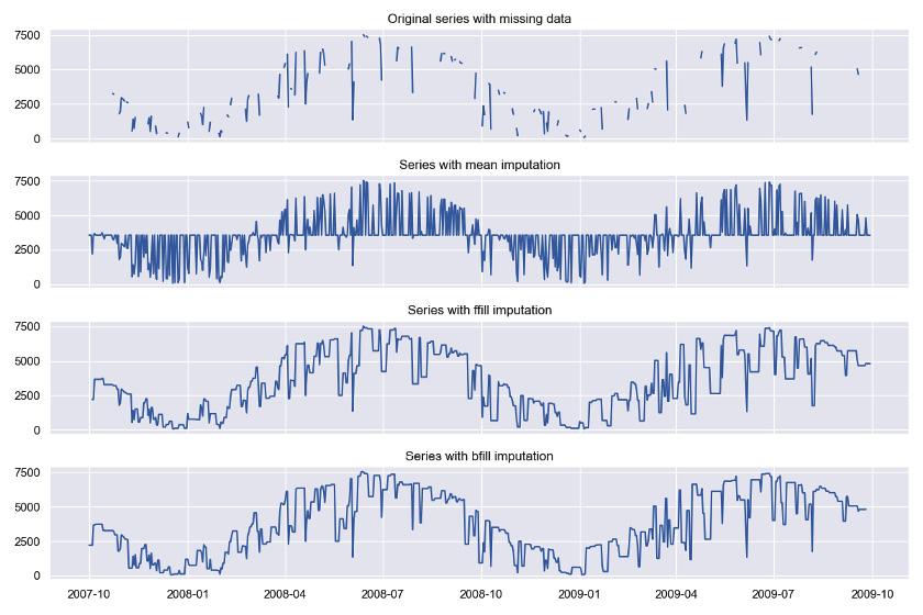
So now, instead of continuously dealing with irregular gaps, we had a much more predictable structure:

ID 1 → 300 points
ID 2 → 300 points
ID 3 → 300 points
...
ID N → 300 points

Here, 300 is just an example based on the chosen time period and sampling interval. Previously, different IDs could have had different numbers of observations, such as 200, 248, 289, or 232, depending on the timestamps that were actually available. This made the data irregular and meant that the amount of work required for each ID could vary.

This regularity made the workload much more predictable and, importantly, gave us a structure that was much easier to process in parallel on the GPU.

10. What Actually Worked

The final improvement did not come from one magical CUDA call.

It came from combining several ideas:

1. Identify operations with enough computational work

Small operations were not automatically worth moving to the GPU. We focused on workloads where parallel execution could make a meaningful difference.

2. Reduce unnecessary chunking

Where the operation allowed it, we provided larger batches of data rather than repeatedly launching small pieces of work.

3. Make the data more regular

Creating a consistent time grid reduced irregularity and gave downstream processing a predictable structure.

4. Separate independent computation from dependent computation

Not every preprocessing operation was a good GPU candidate.

We had to understand which operations could actually execute independently.

5. Keep the computation coherent

Rather than constantly bouncing between CPU and GPU representations, we tried to keep larger portions of the computation together where possible.

                    Workload
                       │
              ┌────────┴────────┐
              ▼                 ▼
        Independent          Dependent
        computation          computation
              │                 │
              ▼                 ▼
             GPU          CPU / suitable
                           execution path

11. The Results

The workload contained approximately:

• ~1 million rows

• ~3,000 unique IDs

• ~300 observations per ID

Initially, the preprocessing stage took approximately:

120 seconds

After the optimization for the preprocessing module:

~10 seconds

That represents:

92% reduction in preprocessing time.

However, preprocessing was not the only component of the pipeline.

Data fetching and other parts of the pipeline also contributed to the total runtime.

A simplified view was approximately:

BEFORE

┌─────────────────────┐
│ Data fetching ~60s  │
├─────────────────────┤
│ Preprocessing ~120s │
└─────────────────────┘
        ~180s

After the optimization, including improvements to the query/fetching path:

AFTER

┌─────────────────────┐
│ Data fetching ~40s  │
├─────────────────────┤
│ GPU processing ~10s │
└─────────────────────┘
         ~50s

So the preprocessing stage itself improved by roughly 92%, while the overall pipeline saw an improvement of roughly 60%+.

12. What I Learned

Profile before optimizing

Don't assume the model is the bottleneck.

Measure where the time actually goes.

GPUs are not automatically faster

The workload matters.

Large, repetitive, parallel computations are where GPUs can shine.

A tiny operation may technically run faster on the GPU and still make almost no difference to the application.

Parallelism requires independence

A large dataset does not automatically mean a highly parallel workload.

Dependencies can limit what can be executed simultaneously.

Batch size matters

Giving a GPU too little work can leave its parallel execution resources underutilized.

But simply making a batch larger isn't enough either. The computation still needs to be parallelizable.

Data movement matters, but context matters more

CPU-GPU transfers have a cost.

But that cost needs to be considered relative to the amount of computation being accelerated.

For a large workload, spending a second moving data may be insignificant if the computation saves tens of seconds.

Regular data is easier to process

Turning irregular time-series data into a consistent representation made the downstream computation easier to reason about and optimize.

13. The Question That Came Next

At this point, I had a much better understanding of when GPU parallelization could help.

But I still had a fundamental question.

I was thinking about the GPU as:

"A device with thousands of cores that can perform lots of operations simultaneously."

That explanation is useful, but incomplete.

What actually happens when we launch work on the GPU?

How does the GPU take something like:

C = A @ B

and distribute that enormous amount of work?

What exactly is a thread? Why are threads grouped into blocks? And why doesn't one thread simply map to one GPU core?

And many more terminologies and questions...

Understanding those concepts changed the way I thought about GPU optimization.

That became the next part of the journey:

From Threads to Warps: Understanding Kernels and how a GPU Actually Executes Work